PI-DSMC Documentation

PI-DSMC V3 (CPU)

4. Configuration

The geometry, the physical properties of the simulation and the boundary conditions are defined using the program graphical user interface called PIDSMCconfig. PIDSMCconfig runs under the X Window System. After starting PIDSMCconfig, the user needs to select the dimensionality of the data set. The main window of PIDSMCconfig in 2D mode and in 3D mode is shown below.

The menu provides load and save commands in the file section as well as configuration dialogs in the setup section. The file extension used for PI-DSMC configuration files is ds2 and ds3 for 2D and 3D data sets respectively.

4.1 Geometry definition

4.1.1 Domain configuration

The geometry definition usually begins with the configuration of the domain. To configure the domain, click on Setup in the menu and select Domain and General. The window shown below will appear.

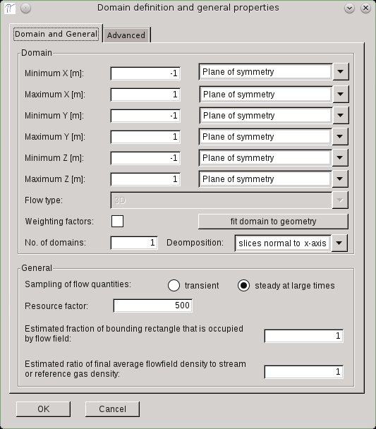
In 2D the flow type can either be planar or axially symmetric. PI-DSMC does not support radial weighting factors. For 2D planar simulations, the minimum and maximum x and y coordinates must be defined.
For 2D axially symmetric simulations the maximum radius (maximum y) must be defined additionally to the minimum and maximum height (x-axis). The x-axis (y = 0) is the axis of rotational symmetry, therefore the minimum y is set to zero.

A boundary condition must be selected for each of the four domain boundaries. The following options are available for all boundaries:

Plane of symmetry: specular reflection of molecules

Interface with the reference gas: molecules enter the simulation domain. The number flux is determined by the parameters of the reference gas.

Interface with the secondary gas: molecules enter the simulation domain. The number flux is determined by the parameters of the secondary gas.

Interface with a vacuum: adsorption of all molecules

Not in the flow: choose this when the complete boundary is inside a body.

In 2D the minimum and maximum x boundaries can be periodic boundaries.
The minimum y axis can be the axis of rotational symmetry in axially symmetric flows. This option is chosen automatically when "axial symmetric flow" is selected.

The resource factor determines the coarseness of the computational grid and the number of real molecules per simulated molecule. For simulations with small density variations the resource factor must be increased, until the quality requirement (mcs/mfp < 1/3) is met everywhere in the flow.

The estimated fraction of bounding rectangle that is occupied by flow field should be adjusted when large areas of the domain are filled with solid.

The estimated ratio of final average flow field density to stream or reference gas density should be adjusted when flows with large pressure gradients are simulated. The number of real molecules represented by each simulated molecule is proportional to this factor.

After the parameters have been entered, the computational domain will be shown in the main window. The grey box represents the domain boundary. Please, note that the view is not to scale.

4.1.2 2D Surface definition

Each individual surface is defined by surface segments. A surface is "open" when the starting point and the end point do not coincide, and "closed" otherwise. Starting and ending points of open surfaces must be located on the domain boundary.
The definition of a single surface begins with the creation of a line primitive. To create a line primitive, click the "Add surface" button at the top of the window. Now, determine the starting point of the line primitive by clicking on a point inside the domain. Determine the ending point by clicking on a second point inside the domain. After that, a straight line and two points will be draw.
Move the mouse above the line primitive. The line will turn red indicating that the line is selected. A circle that moves along the line will appear. The direction of movement indicates the direction of the surface. The gas will always be on the right when looking in the direction of the surface. The left side from the direction of the surface will be solid area.

More complex surfaces can be created by adding intersections to straight line segments. To add an intersection, click the Add intersection button at the top of the screen. Click on a straight line segment to select the line that will be intersected. After that, click on a point inside the domain. This point will connect to the starting point and to the ending point of the selected line segment. A new point will be drawn and a new line segment will be added.

Line segments cannot be deleted. Only connecting points can be deleted. To delete a connecting point, click on Remove intersection. After that, click on the point that you want to remove.

Multiple surfaces can be created by creating multiple surface primitives. A single surface cannot be split into two individual surfaces. The position of connecting points can be edited. Double click on a connecting point to edit its coordinates.

4.1.3 2D Surface segment properties and surface group definition

To edit the properties of a line segment double click on any line segment. The following dialog will appear.

Each line segment must contain at least one sampling interval. Sampling intervals have 2 purposes: First of all, the surface properties are calculated for each sampling interval. Second, the sampling intervals are used to define the surface parameters. Each sampling interval can be assigned different surface properties. The number of sampling intervals therefore determines the spatial resolution of the obtained surface quantities and of the surface parameters.

Each line segment can be either a straight line or a circle segment. The coordinates of the circle center are constrained by the geometry. If one coordinate is entered, the second is computed automatically.

The side that is occupied by the flow can be switched by checking the corresponding check box and clicking OK. The animated circle will now move in the opposite direction which indicates that the direction of the surface was changed. The flow is still to the right side of the direction of the surface! This setting applies to the complete surface, not just to the selected line segment.

The surface is closed when the corresponding check box is checked. A closed surface must contain three points at least.

The properties of the surfaces are defined in groups. Surface groups apply to the complete surface, not just to the selected line segment. To add a new surface group click on add. To edit the properties of the new surface group select the group from the list and click on edit. The following window will appear.

domain configuration

The number of sampling intervals in each group determines the extension of a surface group along the surface. The sample intervals are counted in the direction of the surface, starting from the starting point which is painted in green. All sampling intervals of the surface must be contained in a surface group.

There are three different surface types:

Solid, species independent or species dependent

Flow entry

Stream boundary

A solid surface can have different thermal properties. First of all, the surface can have a fixed uniform temperature. Second, the surface can be adiabatic with a defined minimum temperature and an emissivity. Third, there can be zero heat transfer and infinite thermal conductivity with a specified emissivity. A solid surface can have an in-plan velocity. The y component of this velocity is zero and the velocity vector of each sampling interval is parallel to the surface segments. The velocity in the z direction, i.e. the radial velocity for axially symmetric flows, can be defined separately. The probability of each surface reaction can be defined. The remaining properties of a solid surface can be either species independent or species dependent.

The definition of a flow entry surface is straight forward. The flow is characterized by three velocity components, the temperature, the number density and the fraction of each species.

The stream boundary is similar to the flow entry surface but the parameters are those of the reference gas.

4.1.4 3D Surface definition

In 3D mode the flow geometry is defined by a surface mesh consisting of triangles. PIDSMCconfig provides neither surface mesh generation nor surface mesh editing tools. The user has to generate a surface mesh consisting with an external program.

The surface mesh must be closed and the surface normals must point outwards. Surface triangles are allowed to coincide with the bounding box. The surface mesh can be loaded into PIDSMCconfig by clicking the Add surface button. After clicking the button a file open dialog will appear. The surface mesh must be stored in a file with the extension "dat". The file format is as follows:

1 # all surfaces are treated as one
M # the number of patches that form the complete surface
for j = 1 to M:
N # the number of triangles for patch j N
for k = 1 to N:
X1 Y1 Z1 X2 Y2 Z2 X3 Y3 Z3 # vertices of triangle k
end for
end for

A simple example looks like this:

1 # 1 surface
2 # 2 patches
1 # 1 triangle in path 1
7.0e-2 6.0e-2 -2.0e-2 -1.0e-2 1.0e-1 -1.0e-2 1.0e-2 1.0e-2 8.0e-2
5 # 5 triangles in patch 2
-1.0e-2 1.0e-1 -1.0e-2 0.0e+0 0.0e+0 0.0e+0 1.0e-2 1.0e-2 8.0e-2
0.0e+0 0.0e+0 0.0e+0 7.0e-2 6.0e-2 -2.0e-2 1.0e-2 1.0e-2 8.0e-2
1.0e-2 1.0e-2 -8.0e-2 7.0e-2 6.0e-2 -2.0e-2 0.0e+0 0.0e+0 0.0e+0
1.0e-2 1.0e-2 -8.0e-2 -1.0e-2 1.0e-1 -1.0e-2 7.0e-2 6.0e-2 -2.0e-2
1.0e-2 1.0e-2 -8.0e-2 0.0e+0 0.0e+0 0.0e+0 -1.0e-2 1.0e-1 -1.0e-2

PIDSMCConfig will generate a separate surface group for each surface patch. The properties of the surface groups can be edited as in the 2D case.

4.2 Gas definition

The gas definition consists of the definition of the reference gas, the definition of the molecular species and the definition of the chemical reaction at the surface and in the flow volume. To open the gas definition dialog click on Setup in the main menu and click on Gas.

The definition of the reference gas is straight forward. The required parameters are the number density, the temperature, the vibrational temperature if any species has rotational degrees of freedom, three velocity components and the fraction of each species.

There are two possibilities to define a molecular species. First, the species can be selected from the list of predefined species. Currently, the following species are available: Hard sphere molecule, Maxwell molecule, ideal/real oxygen, ideal/real nitrogen, argon, hydrogen, helium, xenon, nitric oxide, carbon dioxide, carbon monoxide, atomic oxygen and atomic nitrogen. The dialog for the configuration of the gas mixture is shown below.

The second option is to create a new species. Every species requires a reference diameter and a reference temperature according to the Larsen-Borgnakke theory, a VSS parameter, the exponent of the exponential law that describes the temperature dependence of the viscosity, a molecular mass and a description.
Rotation and vibration are optional. For rotation, enter the number of rotational degrees of freedom and the value of the rotational collision number. The rotational collision number can either be a constant or a polynomial. For vibration, enter the number of vibrational modes and the characteristic vibrational temperature and the vibrational collision number for each vibrational mode. The vibrational collision number can either be a constant or an irrational function.

After a predefined species was selected or the parameters of a new species were entered, click the Add to gas button. To edit the properties of a previously added species, select the species from the drop down menu. The parameters of the selected species will be displayed. Change the parameters and click update species. To remove a species click on remove species.

Read on...

Please note: This page applies to PI-DSMC V3 which runs on CPUs.